Neural networks are used on the field of data mining in order to perform classification and regression.
Neural networks are ispired to the human brain that works via associations using neurons.
The neurons are individual processing unit, linked each other via synapses.
The figure hereafter shows the structure of a neural network:
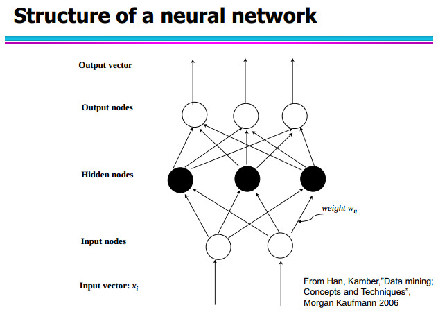
A neural network takes in input a vector containing the record to classify.
It might be composed by more internal levels (the nodes located here are known as “hidden” nodes) and at the end there is a final stage where there is the “exit stage” composed by a number of nodes equal to the number of the class labels. Here each node refers to the “probability” that the examinated record belong to the node’s class label.
Structure of a neuron
As the following figure shows, in a neuron two parameters shall be configured:
- weights vector
- the offset (μk).
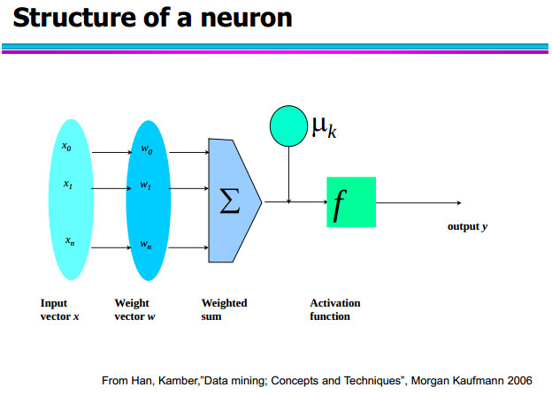
The classification starts doing the scalar product between “x” (input vector) and “w” (weights vector). Afterwards at the outcome value is summed the value of the “offset” and finally is applied an activation function that could be a step, exponential or sinusoidal function.
The output is a value between 0 and 1 and it gives the belonging probability of the record at each output class.
Building a neural network
The building process of a neural network starts from assigning a set of weights and offset in a random way. The next step is to give in input to the neural network the first training set’s record and to see what happens. It turns out that the class label of this record is known (it belongs to the training set!), thus, when the neural network will give in output the belonging’s probability to each class label a process called “Back propagation” starts. Back Propagation (backward propagation of errors) computes the difference or error between the outcome provided and the expected one; it then proceed with a correction of the neuron’s parameters in order to reduce the error. This procedure is repeated for all the training set’s record.
When does the procedure stop?
The stop’s conditions could be:
- when the accurancy of the training set satisfy a defined thresold
- when the correction is too low (a local optimim has been reached)
- when the time elapsed it too high –>too iterations or epocs on the training set.
This approach fits well if there is a continous variable in input of the network since just one entry point will be required. On the contrary, things become more complicated in case of a categorical attribute with high-cardinality in input: in this case an entry point for each domain value is required. If we have to deal with boolean value, it’s straightforward. But for the sake of this demonstation, let’s say that there are attributes such age (which ranges from 0 to 100) and salary (which ranges from 0 to 10.000 £). Those attributes require a pre-processing stage through which they are normalized in a range like [0,1] or [-1,1].
As seen before, operations as product or sum modify data inside the network and their value could go outside the prefigured range. The function called activation function f takes the values back to the right range.
Pros
- hight accurancy (it’s one of the best algorithm)
- Robust also with outliers
- classification is fast
- the output could be discrete or continuos (it is possible to use neural network also for regression)
Cons
- the machine learning process is complex and it could be very slow if the training set is very big (in this case the use of neural network is discouraged)
- the model is not interpretable
- it’s difficult to add new knowledge of the application domain